Доброго времени суток, читатели! Сегодня мы поговорим о матрицах в Matlab, об их применении в решении систем линейных алгебраических уравнений. Подробно разберем методы решения, и для этого необходимо знание нескольких базовых алгоритмов.
Также стоит отметить, что у каждого алгоритма, которым мы будем искать решение СЛАУ в Matlab, своя скорость нахождения этого решения, наличие или отсутствие условия выполнения алгоритма и т.д.
В традициях нашего сайта разберём на примере:
Решить систему линейных уравнений:
4*a + b — c = 6
a — b + c = 4
2*a — 3*b — 3*c = 4
- Метод обратной матрицы в Matlab
- Метод Гаусса
- Метод разложения матрицы
- LU разложение
- QR разложение
- Стандартные функции Matlab
- Повторение
- Решение уравнений и их систем – команда solve
- solve
- Syntax
- Description
- Examples
- Solve Quadratic Equation
- Solve Polynomial and Return Real Solutions
- Numerically Solve Equations
- Solve Multivariate Equations and Assign Outputs to Structure
- Solve Inequalities
- Solve Multivariate Equations and Assign Outputs to Variables
- Use Parameters and Conditions to Refine Solution
- Shorten Result with Simplification Rules
- Ignore Assumptions on Variables
- Solve Polynomial Equations of High Degree
- Return One Solution
- Input Arguments
- eqn — Equation to solve symbolic expression | symbolic equation
- var — Variable for which you solve equation symbolic variable
- eqns — System of equations symbolic expressions | symbolic equations
- vars — Variables for which you solve an equation or system of equations symbolic vector | symbolic matrix
- Name-Value Arguments
- Real — Flag for returning only real solutions false (default) | true
- ReturnConditions — Flag for returning parameters and conditions false (default) | true
- IgnoreAnalyticConstraints — Simplification rules applied to expressions and equations false (default) | true
- IgnoreProperties — Flag for returning solutions inconsistent with properties of variables false (default) | true
- MaxDegree — Maximum degree of polynomial equations for which solver uses explicit formulas 2 (default) | positive integer smaller than 5
- PrincipalValue — Flag for returning one solution false (default) | true
- Output Arguments
- S — Solutions of equation symbolic array
- Y — Solutions of system of equations structure
- y1. yN — Solutions of system of equations symbolic variables
- parameters — Parameters in solution vector of generated parameters
- conditions — Conditions under which solutions are valid vector of symbolic expressions
- Algorithms
Метод обратной матрицы в Matlab
Начнем с достаточно распространенного метода. Его суть состоит в том, что сначала необходимо выписать коэффициенты при a, b и c (то есть те коэффициенты, которые находятся слева) в одну матрицу, а свободный член (то есть то, что справа) в другую.
В итоге у нас получится 2 матрицы:
Для реализации этого метода (и следующих методов тоже) требуется одно условие: чтобы определитель матрицы, составленной из коэффициентов левой части не был равен нулю. Проверка на определитель:
После проверки условия можем перейти к следующему шагу: нахождение обратной матрицы. В Matlab для этого используется оператор inv .
А само решение СЛАУ в Matlab находится как перемножение найденной обратной матрицы на матрицу свободных членов:
Мы получили 3 значения, которые и соответствуют нашим коэффициентам: то есть a = 2, b = -1, c = 1 . Можете проверить, подставив полученные ответы в исходную систему, и убедиться, что мы решили СЛАУ правильно.
Также следует отметить, что матрицы нужно перемножать именно, как сделали мы, то есть слева обратная матрица, справа матрица свободных членов.
Если вы не все поняли, то советую вам почитать нашу статью по основам Matlab.
Метод Гаусса
Метод Гаусса в Matlab реализуется достаточно просто: для этого нам нужно всего лишь изучить один новый оператор.
() — левое деление.
При следующей записи:
Мы получим ответы на нашу исходную систему. Только заметьте, мы решили СЛАУ стандартным набором функций в Matlab, и желательно этот оператор использовать когда матрица коэффициентов квадратная, так как оператор приводит эту матрицу к треугольному виду. В других случаях могут возникнуть ошибки.
Метод разложения матрицы
Теперь поговорим о разложении матрицы. Нахождение решения через разложение матрицы очень эффективно. Эффективность обусловлена скоростью нахождения решения для данного вида систем и точностью полученных результатов.
Возможны следующие разложения:
- разложение Холецкого
- LU разложение
- QR разложение
Разберём решение через LU и QR разложение, так как в задачах чаще всего встречается задание на решение именно через такие разложения.
Основное отличие этих двух разложений: LU разложение применимо только для квадратных матриц, QR — возможно и для прямоугольных.
LU разложение
Решим выше предложенную задачу через LU разложение:
QR разложение
И через QR разложение соответственно:
Отметим, что апостроф ( ‘ ) после Q означает транспонирование.
Стандартные функции Matlab
Так же Matlab предлагает функцию linsolve , с помощью которой возможно решить систему линейных алгебраических уравнений. Выглядит это так:
Как видите, ничего сложного тут нет, на то они и стандартные функции Matlab.
Повторение
Итак, сегодня мы с вами изучили несколько методов для решения СЛАУ в Matlab, как с помощью матриц, так и с помощью стандартных функций. Давайте их повторим на другом примере:
Решить систему линейных уравнений:
6*a — b — c = 0
a — 2*b + 3*d = 0
3*a — 4*b — 4*c = -1
- Методом обратной матрицы:
- Методом Гаусса:
- LU разложение:
- QR разложение:
На этом я с вами попрощаюсь, надеюсь, вы научились применять матрицы в Matlab для решения СЛАУ.
Решение уравнений и их систем – команда solve
Дата добавления: 2015-06-12 ; просмотров: 5230 ; Нарушение авторских прав
Для решения систем уравнений и одиночных уравнений служит команда
solve(expr1, expr2. exprN, var1, var2. varN). Она возвращает значения переменных varI, при которых соблюдаются равенства, заданные выражениями exprI. Если в выражениях не используются знаки равенства, то полагается, что exprI = 0.
Результат может быть возвращен в следующих формах:
для одного уравнения и одной переменной решение возвращается в виде одномерного или многомерного массива ячеек;
при одинаковом числе уравнений и переменных решение возвращается в упорядоченном по именам переменных виде.
Команда solve позволяет найти не только вещественные, но и комплексные решения систем уравнений и одиночных уравнений. Справку по этой команде можно получить, введя команду doc solve.
Решить уравнение x 3 — 1 = 0.
В результате получены три разных значения корня x1 = 1, x2 = , x3 = , которые хранятся соответственно в элементах S(1), S(2), S(3) массива S.
С помощью subs (разд. 7.7) подставим найденные значения корней в выражение x 3 — 1:
Выражение x 3 — 1 принимает значение 0 при подстановке любого из найденных корней, поэтому x1, x2, x3 являются точными корнями уравнения x 3 — 1 = 0.
Команда roots (см. разд. 6.1) нашла бы только приближенные значения корней уравнения x 3 — 1 = 0. В общем случае полиномиальное уравнение степени выше 4 не может иметь точного решения, выраженного с помощью радикалов.
Команда solve позволяет решать уравнения, представленные в аналитическом виде.
Решить квадратное уравнение ax 2 +bx+c = 0.
Команда solve возвратила известные выражения корней x1,2 = квадратного уравнения ax 2 +bx+c = 0. Точно также можно выразить с помощью радикалов решения кубического уравнения ax 3 +bx 2 +cx+d = 0, хотя эти выражения достаточно сложные.
Решить трансцендентное уравнение x lnx +1 — 1 = 0.
В данном случае solve нашла точные значения корней x1 = 1, x2 = e −1 .
Решить трансцендентное уравнение lnx + 3 — x = 0.
Команда solve возвратила значения корней, выраженные через функцию Ламберта.
Команда vpa возвращает приближенные значения этих корней, вычисленные с 20 значащими цифрами:
Каждый из приближенных корней этого уравнения был найден по отдельности в разделе 6.2 с помощью команды fzero. Отметим, что команда solve нашла приближенные значения двух корней одновременно с высокой точностью. При этом не пришлось графически определять интервалы изоляции корней.
Решение любого трансцендентного уравнения, в том числе и тригонометрического (разд. 7.17), достаточно сложная и серьезная проблема. Иногда solve возвращает неверные решения.
Решить трансцендентное уравнение sinx lnsinx +x x — 2 = 0.
Найденное решение неверное, т. к. оно не прошло проверку подстановкой.
Команда solve может возвратить не все решения.
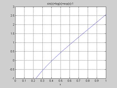
Решить трансцендентное уравнение sinx+lnx+e x — 1 = 0.
Возвратив приближенный комплексный корень уравнения x1 = -3,0553 — 1,7145i, solve не нашла вещественный корень. С помощью команды ezplot (разд. 7.16) графически определяем, что он находится вблизи значения 0,4 (рис. 7.2):
Вещественный корень со стартовым приближением 0,4 найдем с помощью команды fzero(разд. 6.2):
Итак, приближенное значение вещественного корня x2=0,4072.
Перейдем теперь к системам уравнений.
Решить систему уравнений

Результатом выполнения команды solve является структура S с полями x и y, каждое из которых содержит символьное представление решения:
Выведем в командное окно содержимое структуры:
Для проверки подставим в выражения Y1 = x+y — 3 и Y2 = xy 2 — 4 вначале первое решение, а затем второе:
>> disp(subs([Y1 Y2],[x y],[S.x(1) S.y(1)])
>> disp(subs([Y1 Y2],[x y],[S.x(2) S.y(2)])
Как видим, найдены точные решения, т. к. выражения Y1 и Y2 при их подстановке обратились в 0.
Команда solve допускает использование символьных переменных в качестве выходных аргументов. Эквивалентное обращение к solve в предыдущем примере имеет вид:
Команда solve позволяет решать системы уравнений, заданные в аналитическом виде.
Решить систему уравнений относительно x, y, z
solve
Equations and systems solver
Support for character vector or string inputs has been removed. Instead, use syms to declare variables and replace inputs such as solve(‘2*x == 1′,’x’) with solve(2*x == 1,x) .
Syntax
Description
S = solve( eqn , var ) solves the equation eqn for the variable var . If you do not specify var , the symvar function determines the variable to solve for. For example, solve(x + 1 == 2, x) solves the equation x + 1 = 2 for x.
S = solve( eqn , var , Name,Value ) uses additional options specified by one or more Name,Value pair arguments.
Y = solve( eqns , vars ) solves the system of equations eqns for the variables vars and returns a structure that contains the solutions. If you do not specify vars , solve uses symvar to find the variables to solve for. In this case, the number of variables that symvar finds is equal to the number of equations eqns .
Y = solve( eqns , vars , Name,Value ) uses additional options specified by one or more Name,Value pair arguments.
[ y1. yN ] = solve( eqns , vars ) solves the system of equations eqns for the variables vars . The solutions are assigned to the variables y1. yN . If you do not specify the variables, solve uses symvar to find the variables to solve for. In this case, the number of variables that symvar finds is equal to the number of output arguments N .
[ y1. yN ] = solve( eqns , vars , Name,Value ) uses additional options specified by one or more Name,Value pair arguments.
[ y1. yN , parameters , conditions ] = solve( eqns , vars ,’ ReturnConditions ‘,true) returns the additional arguments parameters and conditions that specify the parameters in the solution and the conditions on the solution.
Examples
Solve Quadratic Equation
Solve the quadratic equation without specifying a variable to solve for. solve chooses x to return the solution.
Specify the variable to solve for and solve the quadratic equation for a .
Solve Polynomial and Return Real Solutions
Solve a fifth-degree polynomial. It has five solutions.
Return only real solutions by setting ‘Real’ option to true . The only real solutions of this equation is 5 .
Numerically Solve Equations
When solve cannot symbolically solve an equation, it tries to find a numeric solution using vpasolve . The vpasolve function returns the first solution found.
Try solving the following equation. solve returns a numeric solution because it cannot find a symbolic solution.
Plot the left and the right sides of the equation. Observe that the equation also has a positive solution.
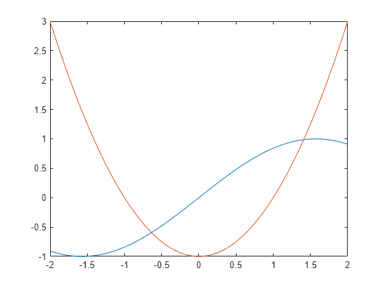
Find the other solution by directly calling the numeric solver vpasolve and specifying the interval.
Solve Multivariate Equations and Assign Outputs to Structure
When solving for multiple variables, it can be more convenient to store the outputs in a structure array than in separate variables. The solve function returns a structure when you specify a single output argument and multiple outputs exist.
Solve a system of equations to return the solutions in a structure array.
Access the solutions by addressing the elements of the structure.
Using a structure array allows you to conveniently substitute solutions into other expressions.
Use the subs function to substitute the solutions S into other expressions.
If solve returns an empty object, then no solutions exist.
Solve Inequalities
The solve function can solve inequalities and return solutions that satisfy the inequalities. Solve the following inequalities.
x 2 + y 2 + x y 1
Set ‘ReturnConditions’ to true to return any parameters in the solution and conditions on the solution.
The parameters u and v do not exist in MATLAB® workspace and must be accessed using S.parameters .
Check if the values u = 7/2 and v = 1/2 satisfy the condition using subs and isAlways .
isAlways returns logical 1 ( true ) indicating that these values satisfy the condition. Substitute these parameter values into S.x and S.y to find a solution for x and y .
Solve Multivariate Equations and Assign Outputs to Variables
Solve the system of equations.
When solving for more than one variable, the order in which you specify the variables defines the order in which the solver returns the solutions. Assign the solutions to variables solv and solu by specifying the variables explicitly. The solver returns an array of solutions for each variable.
Entries with the same index form the pair of solutions.
Use Parameters and Conditions to Refine Solution
Return the complete solution of an equation with parameters and conditions of the solution by specifying ‘ReturnConditions’ as true .
Solve the equation sin ( x ) = 0 . Provide two additional output variables for output arguments parameters and conditions .
The solution π k contains the parameter k , where k must be an integer. The variable k does not exist in MATLAB workspace and must be accessed using parameters .
Restrict the solution to 0 x 2 π . Find a valid value of k for this restriction. Assume the condition, conditions , and use solve to find k . Substitute the value of k found into the solution for x .
Alternatively, determine the solution for x by choosing a value of k . Check if the value chosen satisfies the condition on k using isAlways .
Check if k = 4 satisfies the condition on k .
isAlways returns logical 1( true ), meaning that 4 is a valid value for k . Substitute k with 4 to obtain a solution for x . Use vpa to obtain a numeric approximation.
Shorten Result with Simplification Rules
Solve the equation exp ( log ( x ) log ( 3 x ) ) = 4 .
By default, solve does not apply simplifications that are not valid for all values of x . In this case, the solver does not assume that x is a positive real number, so it does not apply the logarithmic identity log ( 3 x ) = log ( 3 ) + log ( x ) . As a result, solve cannot solve the equation symbolically.
Set ‘IgnoreAnalyticConstraints’ to true to apply simplification rules that might allow solve to find a solution. For details, see Algorithms.
solve applies simplifications that allow the solver to find a solution. The mathematical rules applied when performing simplifications are not always valid in general. In this example, the solver applies logarithmic identities with the assumption that x is a positive real number. Therefore, the solutions found in this mode should be verified.
Ignore Assumptions on Variables
The sym and syms functions let you set assumptions for symbolic variables.
Assume that the variable x is positive.
When you solve an equation for a variable under assumptions, the solver only returns solutions consistent with the assumptions. Solve this equation for x .
Allow solutions that do not satisfy the assumptions by setting ‘IgnoreProperties’ to true .
For further computations, clear the assumption that you set on the variable x by recreating it using syms .
Solve Polynomial Equations of High Degree
When you solve a polynomial equation, the solver might use root to return the solutions. Solve a third-degree polynomial.
Try to get an explicit solution for such equations by calling the solver with ‘MaxDegree’ . The option specifies the maximum degree of polynomials for which the solver tries to return explicit solutions. The default value is 2 . Increasing this value, you can get explicit solutions for higher order polynomials.
Solve the same equations for explicit solutions by increasing the value of ‘MaxDegree’ to 3 .
Return One Solution
Solve the equation sin ( x ) + cos ( 2 x ) = 1 .
Instead of returning an infinite set of periodic solutions, the solver picks three solutions that it considers to be the most practical.
Choose only one solution by setting ‘PrincipalValue’ to true .
Input Arguments
eqn — Equation to solve
symbolic expression | symbolic equation
Equation to solve, specified as a symbolic expression or symbolic equation. The relation operator == defines symbolic equations. If eqn is a symbolic expression (without the right side), the solver assumes that the right side is 0, and solves the equation eqn == 0 .
var — Variable for which you solve equation
symbolic variable
Variable for which you solve an equation, specified as a symbolic variable. By default, solve uses the variable determined by symvar .
eqns — System of equations
symbolic expressions | symbolic equations
System of equations, specified as symbolic expressions or symbolic equations. If any elements of eqns are symbolic expressions (without the right side), solve equates the element to 0 .
vars — Variables for which you solve an equation or system of equations
symbolic vector | symbolic matrix
Variables for which you solve an equation or system of equations, specified as a symbolic vector or symbolic matrix. By default, solve uses the variables determined by symvar .
The order in which you specify these variables defines the order in which the solver returns the solutions.
Name-Value Arguments
Real — Flag for returning only real solutions
false (default) | true
Flag for returning only real solutions, specified as the comma-separated pair consisting of ‘Real’ and one of these values.
| false | Return all solutions. |
| true | Return only those solutions for which every subexpression of the original equation represents a real number. This option also assumes that all symbolic parameters of an equation represent real numbers. |
ReturnConditions — Flag for returning parameters and conditions
false (default) | true
Flag for returning parameters in solution and conditions under which the solution is true, specified as the comma-separated pair consisting of ‘ReturnConditions’ and one of these values.
| false | Do not return parameterized solutions and the conditions under which the solution holds. The solve function replaces parameters with appropriate values. |
| true | Return the parameters in the solution and the conditions under which the solution holds. For a call with a single output variable, solve returns a structure with the fields parameters and conditions . For multiple output variables, solve assigns the parameters and conditions to the last two output variables. This behavior means that the number of output variables must be equal to the number of variables to solve for plus two. |
Example: [v1, v2, params, conditions] = solve(sin(x) +y == 0,y^2 == 3,’ReturnConditions’,true) returns the parameters in params and conditions in conditions .
IgnoreAnalyticConstraints — Simplification rules applied to expressions and equations
false (default) | true
Simplification rules applied to expressions and equations, specified as the comma-separated pair consisting of ‘IgnoreAnalyticConstraints’ and one of these values.
| false | Use strict simplification rules. |
| true | Apply purely algebraic simplifications to expressions and equations. Setting IgnoreAnalyticConstraints to true can give you simpler solutions, which could lead to results not generally valid. In other words, this option applies mathematical identities that are convenient, but the results might not hold for all possible values of the variables. In some cases, it also enables solve to solve equations and systems that cannot be solved otherwise. |
IgnoreProperties — Flag for returning solutions inconsistent with properties of variables
false (default) | true
Flag for returning solutions inconsistent with the properties of variables, specified as the comma-separated pair consisting of ‘IgnoreProperties’ and one of these values.
| false | Do not include solutions inconsistent with the properties of variables. |
| true | Include solutions inconsistent with the properties of variables. |
MaxDegree — Maximum degree of polynomial equations for which solver uses explicit formulas
2 (default) | positive integer smaller than 5
Maximum degree of polynomial equations for which solver uses explicit formulas, specified as a positive integer smaller than 5. The solver does not use explicit formulas that involve radicals when solving polynomial equations of a degree larger than the specified value.
PrincipalValue — Flag for returning one solution
false (default) | true
Flag for returning one solution, specified as the comma-separated pair consisting of ‘PrincipalValue’ and one of these values.
| false | Return all solutions. |
| true | Return only one solution. If an equation or a system of equations does not have a solution, the solver returns an empty symbolic object. |
Output Arguments
S — Solutions of equation
symbolic array
Solutions of an equation, returned as a symbolic array. The size of a symbolic array corresponds to the number of the solutions.
Y — Solutions of system of equations
structure
Solutions of a system of equations, returned as a structure. The number of fields in the structure correspond to the number of independent variables in a system. If ‘ReturnConditions’ is set to true , the solve function returns two additional fields that contain the parameters in the solution, and the conditions under which the solution is true.
y1. yN — Solutions of system of equations
symbolic variables
Solutions of a system of equations, returned as symbolic variables. The number of output variables or symbolic arrays must be equal to the number of independent variables in a system. If you explicitly specify independent variables vars , then the solver uses the same order to return the solutions. If you do not specify vars , the toolbox sorts independent variables alphabetically, and then assigns the solutions for these variables to the output variables.
parameters — Parameters in solution
vector of generated parameters
Parameters in a solution, returned as a vector of generated parameters. This output argument is only returned if ReturnConditions is true . If a single output argument is provided, parameters is returned as a field of a structure. If multiple output arguments are provided, parameters is returned as the second-to-last output argument. The generated parameters do not appear in the MATLAB ® workspace. They must be accessed using parameters .
Example: [solx, params, conditions] = solve(sin(x) == 0, ‘ReturnConditions’, true) returns the parameter k in the argument params .
conditions — Conditions under which solutions are valid
vector of symbolic expressions
Conditions under which solutions are valid, returned as a vector of symbolic expressions. This output argument is only returned if ReturnConditions is true . If a single output argument is provided, conditions is returned as a field of a structure. If multiple output arguments are provided, conditions is returned as the last output argument.
Example: [solx, params, conditions] = solve(sin(x) == 0, ‘ReturnConditions’, true) returns the condition in(k, ‘integer’) in conditions . The solution in solx is valid only under this condition.
If solve cannot find a solution and ReturnConditions is false , the solve function internally calls the numeric solver vpasolve that tries to find a numeric solution. For polynomial equations and systems without symbolic parameters, the numeric solver returns all solutions. For nonpolynomial equations and systems without symbolic parameters, the numeric solver returns only one solution (if a solution exists).
If solve cannot find a solution and ReturnConditions is true , solve returns an empty solution with a warning. If no solutions exist, solve returns an empty solution without a warning.
If the solution contains parameters and ReturnConditions is true , solve returns the parameters in the solution and the conditions under which the solutions are true. If ReturnConditions is false , the solve function either chooses values of the parameters and returns the corresponding results, or returns parameterized solutions without choosing particular values. In the latter case, solve also issues a warning indicating the values of parameters in the returned solutions.
If a parameter does not appear in any condition, it means the parameter can take any complex value.
The output of solve can contain parameters from the input equations in addition to parameters introduced by solve .
Parameters introduced by solve do not appear in the MATLAB workspace. They must be accessed using the output argument that contains them. Alternatively, to use the parameters in the MATLAB workspace use syms to initialize the parameter. For example, if the parameter is k , use syms k .
The variable names parameters and conditions are not allowed as inputs to solve .
To solve differential equations, use the dsolve function.
When solving a system of equations, always assign the result to output arguments. Output arguments let you access the values of the solutions of a system.
MaxDegree only accepts positive integers smaller than 5 because, in general, there are no explicit expressions for the roots of polynomials of degrees higher than 4.
The output variables y1. yN do not specify the variables for which solve solves equations or systems. If y1. yN are the variables that appear in eqns , then there is no guarantee that solve(eqns) will assign the solutions to y1. yN using the correct order. Thus, when you run [b,a] = solve(eqns) , you might get the solutions for a assigned to b and vice versa.
To ensure the order of the returned solutions, specify the variables vars . For example, the call [b,a] = solve(eqns,b,a) assigns the solutions for a to a and the solutions for b to b .
Algorithms
When you use IgnoreAnalyticConstraints , the solver applies these rules to the expressions on both sides of an equation.
log( a) + log( b) = log( a· b) for all values of a and b. In particular, the following equality is valid for all values of a, b, and c:
log( a b ) = b·log( a) for all values of a and b. In particular, the following equality is valid for all values of a, b, and c:
If f and g are standard mathematical functions and f( g( x)) = x for all small positive numbers, f( g( x)) = x is assumed to be valid for all complex values x. In particular:
asinh(sinh( x)) = x , acosh(cosh( x)) = x , atanh(tanh( x)) = x
W k( x· e x ) = x for all branch indices k of the Lambert W function.
The solver can multiply both sides of an equation by any expression except 0 .
The solutions of polynomial equations must be complete.