Решение нелинейных уравнений в matlab примеры

Видео:Решение системы нелинейных уравнений. Урок 139Скачать

Решение нелинейных уравнений в Matlab

Доброго времени суток. В этой статье мы разберем решение простых нелинейных уравнений с помощью средств Matlab. Посмотрим в действии как стандартные функции, так и сами запрограммируем три распространенных метода для решения нелинейных уравнений.

Общая информация

Уравнения, которые содержат переменные, находящиеся в степенях, отличающихся от единицы, или имеющие нелинейные математические выражения (корень, экспонента, логарифм, синус, косинус и т.д.), а также имеющие вид f(x) = 0 называются нелинейными. В зависимости от сложности такого уравнения применяют методы для решения нелинейных уравнений.

В этой статье, помимо стандартных функций Matlab, мы рассмотрим следующие методы:

• Метод перебора
• Метод простых итераций
• Метод половинного деления

Рассмотрим коротко их алгоритмы и применим для решения конкретной задачи.

Стандартные функции Matlab

Для решения нелинейных уравнений в Matlab есть функция fzero. Она принимает в качестве аргументов саму функцию, которую решаем, и отрезок, на котором происходит поиск корней нелинейного уравнения.

И сразу же разберем пример:

Решить нелинейное уравнение x = exp(-x), предварительно определив интервалы, на которых существуют решения уравнения.

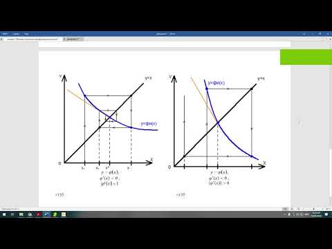
Итак, для начала следует привести уравнение к нужному виду: x — exp(-x) = 0 , а затем определить интервалы, в которых будем искать решение уравнения. Методов для определения интервалов множество, но так как пример достаточно прост мы воспользуемся графическим методом.

Здесь задали примерные границы по оси x, чтобы можно было построить график и посмотреть как ведет себя функция. Вот график:

Из графика видно, что на отрезке [0;1] есть корень уравнения (там, где y = 0), соответственно в дальнейшем будем использовать этот интервал. Чем точнее выбран интервал, тем быстрее метод придет к решению уравнения, а для сложных уравнений правильный выбор интервала определяет погрешность, с которой будет получен ответ.

С помощью стандартной функции Matlab находим корень нелинейного уравнения и выводим. Теперь для проверки отобразим все это графически:

Как вы видите, все достаточно точно просчиталось. Теперь мы исследуем эту же функцию с помощью других методов и сравним полученные результаты.

Метод перебора Matlab

Самый простой метод, который заключается в том, что сначала задается какое то приближение x (желательно слева от предполагаемого корня) и значение шага h. Затем, пока выполняется условие f(x) * f(x + h) > 0, значение x увеличивается на значение шага x = x + h. Как только условие перестало выполняться — это значит, что решение нелинейного уравнения находится на интервале [x; x + h].

Теперь реализуем метод перебора в Matlab:

Лучше всего создать новый m-файл, в котором и прописать код. После вызова получаем такой вывод:

Функцию объявляем с помощью очень полезной команды inline, в цикле пока выполняется условие отсутствия корней (или их четного количества), прибавляем к x значение шага. Очевидно, что чем точнее начальное приближение, тем меньше итераций необходимо затратить.

Метод простых итераций Matlab

Этот метод заключается в том, что функцию преобразуют к виду: x = g(x). Эти преобразования можно сделать разными способами, в зависимости от вида начальной функции. Помимо этого следует задать интервал, в котором и будет производиться итерационный процесс, а также начальное приближение. Сам процесс строится по схеме x_n= g(x_n-1). То есть итерационно проходим от предыдущего значения к последующему.

Процесс заканчивается как только выполнится условие: , то есть, как только будет достигнута заданная точность. И сразу же разберем реализацию метода простых итераций в Matlab для примера, который был приведен выше.

Здесь должно быть все понятно, кроме одного: зачем задавать число итераций? Это нужно для того, чтобы программа не зацикливалась и не выполняла ненужные итерации, а также потому что не всегда программа может просчитать решение с нужной точностью — поэтому следует ограничивать число итераций.

А вот и вывод программы:

Очевидно, что метод простых итераций работает гораздо быстрее и получает точное решение.

Метод половинного деления Matlab

Метод достаточно прост: существует отрезок поиска решения [a;b], сначала находят значение функции в точке середины c, где c = (a+b)/2. Затем сравнивают знаки f(a) и f(c). Если знаки разные — то решение находится на отрезке [a;c], если нет — то решение находится на отрезке [c;b]. Таким образом мы сократили область в 2 раза. Такое сокращение происходит и дальше, пока не достигнем заданной точности.

Перейдем к реализации метода в Matlab:

Все самое важное происходит в цикле: последовательно сокращаем область нахождения решения, пока не будет достигнута заданная точность.
Вот что получилось в выводе:

Этот метод хорошо работает, когда правильно определен интервал, на котором находится решение. Тем не менее, метод простых итераций считается наиболее точным и быстрым.

Заключение

Сегодня мы рассмотрели решение нелинейных уравнений в Matlab. Теперь нам известны методы перебора, половинного деления, простых итераций. А также, когда нам не важно реализация метода, то можно использовать стандартную функцию в Matlab.

На этом все — спасибо за внимание. В следующей статье мы разберем решение систем нелинейных уравнений в matlab.

Видео:Метод Ньютона (метод касательных) Пример РешенияСкачать

fsolve

Solve system of nonlinear equations

Видео:1 - Решение систем нелинейных уравнений в MatlabСкачать

Syntax

Видео:ТАУ. Matlab/SIMULINK Фазовые портреты систем нелинейных диф. уравненийСкачать

Description

Nonlinear system solver

Solves a problem specified by

for x, where F( x) is a function that returns a vector value.

x is a vector or a matrix; see Matrix Arguments.

x = fsolve( fun , x0 ) starts at x0 and tries to solve the equations fun(x) = 0, an array of zeros.

Note

Passing Extra Parameters explains how to pass extra parameters to the vector function fun(x) , if necessary. See Solve Parameterized Equation.

x = fsolve( fun , x0 , options ) solves the equations with the optimization options specified in options . Use optimoptions to set these options.

x = fsolve( problem ) solves problem , a structure described in problem .

[ x , fval ] = fsolve( ___ ) , for any syntax, returns the value of the objective function fun at the solution x .

[ x , fval , exitflag , output ] = fsolve( ___ ) additionally returns a value exitflag that describes the exit condition of fsolve , and a structure output with information about the optimization process.

[ x , fval , exitflag , output , jacobian ] = fsolve( ___ ) returns the Jacobian of fun at the solution x .

Видео:1 3 Решение нелинейных уравнений методом простых итерацийСкачать

Examples

Solution of 2-D Nonlinear System

This example shows how to solve two nonlinear equations in two variables. The equations are

Convert the equations to the form .

Write a function that computes the left-hand side of these two equations.

Save this code as a file named root2d.m on your MATLAB® path.

Solve the system of equations starting at the point [0,0] .

Solution with Nondefault Options

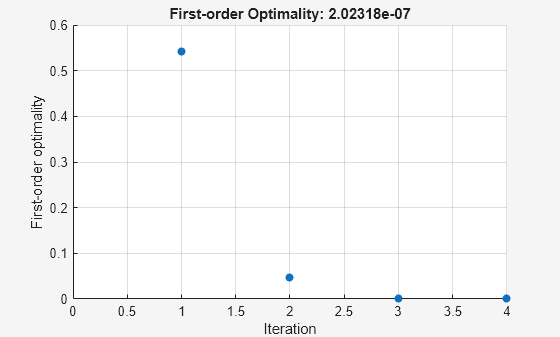
Examine the solution process for a nonlinear system.

Set options to have no display and a plot function that displays the first-order optimality, which should converge to 0 as the algorithm iterates.

The equations in the nonlinear system are

Convert the equations to the form .

Write a function that computes the left-hand side of these two equations.

Save this code as a file named root2d.m on your MATLAB® path.

Solve the nonlinear system starting from the point [0,0] and observe the solution process.

Solve Parameterized Equation

You can parameterize equations as described in the topic Passing Extra Parameters. For example, the paramfun helper function at the end of this example creates the following equation system parameterized by c :

2 x 1 + x 2 = exp ( c x 1 ) — x 1 + 2 x 2 = exp ( c x 2 ) .

To solve the system for a particular value, in this case c = — 1 , set c in the workspace and create an anonymous function in x from paramfun .

Solve the system starting from the point x0 = [0 1] .

To solve for a different value of c , enter c in the workspace and create the fun function again, so it has the new c value.

This code creates the paramfun helper function.

Solve a Problem Structure

Create a problem structure for fsolve and solve the problem.

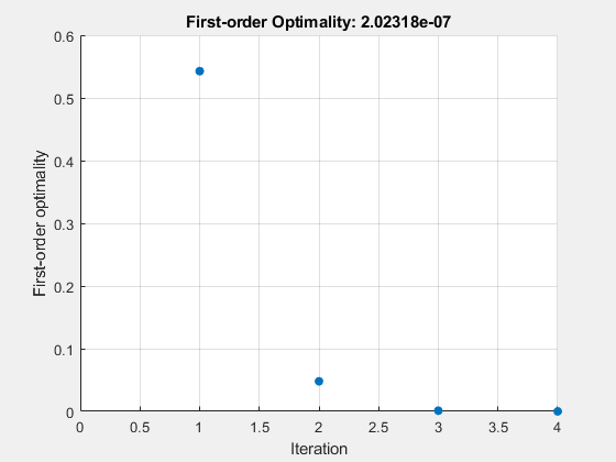
Solve the same problem as in Solution with Nondefault Options, but formulate the problem using a problem structure.

Set options for the problem to have no display and a plot function that displays the first-order optimality, which should converge to 0 as the algorithm iterates.

The equations in the nonlinear system are

Convert the equations to the form .

Write a function that computes the left-hand side of these two equations.

Save this code as a file named root2d.m on your MATLAB® path.

Create the remaining fields in the problem structure.

Solve the problem.

Solution Process of Nonlinear System

This example returns the iterative display showing the solution process for the system of two equations and two unknowns

2 x 1 — x 2 = e — x 1 — x 1 + 2 x 2 = e — x 2 .

Rewrite the equations in the form F ( x ) = 0 :

2 x 1 — x 2 — e — x 1 = 0 — x 1 + 2 x 2 — e — x 2 = 0 .

Start your search for a solution at x0 = [-5 -5] .

First, write a function that computes F , the values of the equations at x .

Create the initial point x0 .

Set options to return iterative display.

Solve the equations.

The iterative display shows f(x) , which is the square of the norm of the function F(x) . This value decreases to near zero as the iterations proceed. The first-order optimality measure likewise decreases to near zero as the iterations proceed. These entries show the convergence of the iterations to a solution. For the meanings of the other entries, see Iterative Display.

The fval output gives the function value F(x) , which should be zero at a solution (to within the FunctionTolerance tolerance).

Examine Matrix Equation Solution

Find a matrix X that satisfies

X * X * X = [ 1 2 3 4 ] ,

starting at the point x0 = [1,1;1,1] . Create an anonymous function that calculates the matrix equation and create the point x0 .

Set options to have no display.

Examine the fsolve outputs to see the solution quality and process.

The exit flag value 1 indicates that the solution is reliable. To verify this manually, calculate the residual (sum of squares of fval) to see how close it is to zero.

This small residual confirms that x is a solution.

You can see in the output structure how many iterations and function evaluations fsolve performed to find the solution.

Видео:Метод простых итераций пример решения нелинейных уравненийСкачать

Input Arguments

fun — Nonlinear equations to solve
function handle | function name

Nonlinear equations to solve, specified as a function handle or function name. fun is a function that accepts a vector x and returns a vector F , the nonlinear equations evaluated at x . The equations to solve are F = 0 for all components of F . The function fun can be specified as a function handle for a file

where myfun is a MATLAB ® function such as

fun can also be a function handle for an anonymous function.

fsolve passes x to your objective function in the shape of the x0 argument. For example, if x0 is a 5-by-3 array, then fsolve passes x to fun as a 5-by-3 array.

If the Jacobian can also be computed and the ‘SpecifyObjectiveGradient’ option is true , set by

the function fun must return, in a second output argument, the Jacobian value J , a matrix, at x .

If fun returns a vector (matrix) of m components and x has length n , where n is the length of x0 , the Jacobian J is an m -by- n matrix where J(i,j) is the partial derivative of F(i) with respect to x(j) . (The Jacobian J is the transpose of the gradient of F .)

Example: fun = @(x)x*x*x-[1,2;3,4]

Data Types: char | function_handle | string

x0 — Initial point
real vector | real array

Initial point, specified as a real vector or real array. fsolve uses the number of elements in and size of x0 to determine the number and size of variables that fun accepts.

Example: x0 = [1,2,3,4]

Data Types: double

options — Optimization options
output of optimoptions | structure as optimset returns

Optimization options, specified as the output of optimoptions or a structure such as optimset returns.

Some options apply to all algorithms, and others are relevant for particular algorithms. See Optimization Options Reference for detailed information.

Some options are absent from the optimoptions display. These options appear in italics in the following table. For details, see View Options.

Choose between ‘trust-region-dogleg’ (default), ‘trust-region’ , and ‘levenberg-marquardt’ .

The Algorithm option specifies a preference for which algorithm to use. It is only a preference because for the trust-region algorithm, the nonlinear system of equations cannot be underdetermined; that is, the number of equations (the number of elements of F returned by fun ) must be at least as many as the length of x . Similarly, for the trust-region-dogleg algorithm, the number of equations must be the same as the length of x . fsolve uses the Levenberg-Marquardt algorithm when the selected algorithm is unavailable. For more information on choosing the algorithm, see Choosing the Algorithm.

To set some algorithm options using optimset instead of optimoptions :

Algorithm — Set the algorithm to ‘trust-region-reflective’ instead of ‘trust-region’ .

InitDamping — Set the initial Levenberg-Marquardt parameter λ by setting Algorithm to a cell array such as .

Display diagnostic information about the function to be minimized or solved. The choices are ‘on’ or the default ‘off’ .

Maximum change in variables for finite-difference gradients (a positive scalar). The default is Inf .

Minimum change in variables for finite-difference gradients (a positive scalar). The default is 0 .

‘off’ or ‘none’ displays no output.

‘iter’ displays output at each iteration, and gives the default exit message.

‘iter-detailed’ displays output at each iteration, and gives the technical exit message.

‘final’ (default) displays just the final output, and gives the default exit message.

‘final-detailed’ displays just the final output, and gives the technical exit message.

Scalar or vector step size factor for finite differences. When you set FiniteDifferenceStepSize to a vector v , the forward finite differences delta are

For optimset , the name is FinDiffRelStep . See Current and Legacy Option Names.

Finite differences, used to estimate gradients, are either ‘forward’ (default), or ‘central’ (centered). ‘central’ takes twice as many function evaluations, but should be more accurate.

The algorithm is careful to obey bounds when estimating both types of finite differences. So, for example, it could take a backward, rather than a forward, difference to avoid evaluating at a point outside bounds.

For optimset , the name is FinDiffType . See Current and Legacy Option Names.

Termination tolerance on the function value, a positive scalar. The default is 1e-6 . See Tolerances and Stopping Criteria.

For optimset , the name is TolFun . See Current and Legacy Option Names.

Check whether objective function values are valid. ‘on’ displays an error when the objective function returns a value that is complex , Inf , or NaN . The default, ‘off’ , displays no error.

Maximum number of function evaluations allowed, a positive integer. The default is 100*numberOfVariables . See Tolerances and Stopping Criteria and Iterations and Function Counts.

For optimset , the name is MaxFunEvals . See Current and Legacy Option Names.

Maximum number of iterations allowed, a positive integer. The default is 400 . See Tolerances and Stopping Criteria and Iterations and Function Counts.

For optimset , the name is MaxIter . See Current and Legacy Option Names.

Termination tolerance on the first-order optimality (a positive scalar). The default is 1e-6 . See First-Order Optimality Measure.

Internally, the ‘levenberg-marquardt’ algorithm uses an optimality tolerance (stopping criterion) of 1e-4 times FunctionTolerance and does not use OptimalityTolerance .

Specify one or more user-defined functions that an optimization function calls at each iteration. Pass a function handle or a cell array of function handles. The default is none ( [] ). See Output Function and Plot Function Syntax.

Plots various measures of progress while the algorithm executes; select from predefined plots or write your own. Pass a built-in plot function name, a function handle, or a cell array of built-in plot function names or function handles. For custom plot functions, pass function handles. The default is none ( [] ):

‘optimplotx’ plots the current point.

‘optimplotfunccount’ plots the function count.

‘optimplotfval’ plots the function value.

‘optimplotstepsize’ plots the step size.

‘optimplotfirstorderopt’ plots the first-order optimality measure.

Custom plot functions use the same syntax as output functions. See Output Functions for Optimization Toolbox™ and Output Function and Plot Function Syntax.

For optimset , the name is PlotFcns . See Current and Legacy Option Names.

If true , fsolve uses a user-defined Jacobian (defined in fun ), or Jacobian information (when using JacobianMultiplyFcn ), for the objective function. If false (default), fsolve approximates the Jacobian using finite differences.

For optimset , the name is Jacobian and the values are ‘on’ or ‘off’ . See Current and Legacy Option Names.

Termination tolerance on x , a positive scalar. The default is 1e-6 . See Tolerances and Stopping Criteria.

For optimset , the name is TolX . See Current and Legacy Option Names.

Typical x values. The number of elements in TypicalX is equal to the number of elements in x0 , the starting point. The default value is ones(numberofvariables,1) . fsolve uses TypicalX for scaling finite differences for gradient estimation.

The trust-region-dogleg algorithm uses TypicalX as the diagonal terms of a scaling matrix.

When true , fsolve estimates gradients in parallel. Disable by setting to the default, false . See Parallel Computing.

Jacobian multiply function, specified as a function handle. For large-scale structured problems, this function computes the Jacobian matrix product J*Y , J’*Y , or J’*(J*Y) without actually forming J . The function is of the form

where Jinfo contains a matrix used to compute J*Y (or J’*Y , or J’*(J*Y) ). The first argument Jinfo must be the same as the second argument returned by the objective function fun , for example, in

Y is a matrix that has the same number of rows as there are dimensions in the problem. flag determines which product to compute:

If flag == 0 , W = J’*(J*Y) .

If flag > 0 , W = J*Y .

In each case, J is not formed explicitly. fsolve uses Jinfo to compute the preconditioner. See Passing Extra Parameters for information on how to supply values for any additional parameters jmfun needs.

Note

‘SpecifyObjectiveGradient’ must be set to true for fsolve to pass Jinfo from fun to jmfun .

For optimset , the name is JacobMult . See Current and Legacy Option Names.

Sparsity pattern of the Jacobian for finite differencing. Set JacobPattern(i,j) = 1 when fun(i) depends on x(j) . Otherwise, set JacobPattern(i,j) = 0 . In other words, JacobPattern(i,j) = 1 when you can have ∂ fun(i) /∂ x(j) ≠ 0.

Use JacobPattern when it is inconvenient to compute the Jacobian matrix J in fun , though you can determine (say, by inspection) when fun(i) depends on x(j) . fsolve can approximate J via sparse finite differences when you give JacobPattern .

In the worst case, if the structure is unknown, do not set JacobPattern . The default behavior is as if JacobPattern is a dense matrix of ones. Then fsolve computes a full finite-difference approximation in each iteration. This can be very expensive for large problems, so it is usually better to determine the sparsity structure.

Maximum number of PCG (preconditioned conjugate gradient) iterations, a positive scalar. The default is max(1,floor(numberOfVariables/2)) . For more information, see Equation Solving Algorithms.

Upper bandwidth of preconditioner for PCG, a nonnegative integer. The default PrecondBandWidth is Inf , which means a direct factorization (Cholesky) is used rather than the conjugate gradients (CG). The direct factorization is computationally more expensive than CG, but produces a better quality step towards the solution. Set PrecondBandWidth to 0 for diagonal preconditioning (upper bandwidth of 0). For some problems, an intermediate bandwidth reduces the number of PCG iterations.

Determines how the iteration step is calculated. The default, ‘factorization’ , takes a slower but more accurate step than ‘cg’ . See Trust-Region Algorithm.

Termination tolerance on the PCG iteration, a positive scalar. The default is 0.1 .

Initial value of the Levenberg-Marquardt parameter, a positive scalar. Default is 1e-2 . For details, see Levenberg-Marquardt Method.

‘jacobian’ can sometimes improve the convergence of a poorly scaled problem. The default is ‘none’ .

Example: options = optimoptions(‘fsolve’,’FiniteDifferenceType’,’central’)

📹 Видео

Решение нелинейных уравненийСкачать

MatLab. 8.8. Решение большой системы нелинейных уравненийСкачать

MatLab. 8.4b. Решение нелинейных задачСкачать

МЗЭ 2021 Лекция 11 Метод Ньютона для решения систем нелинейных уравненийСкачать

2 - Решениt систем линейных алгебраических уравнений (СЛАУ) с помощью Matlab.Скачать

Решение систем Д/У: 1. Знакомство с функциями odeXYСкачать

Компьютерное моделирование - Решение систем нелинейных уравненийСкачать

Метод половинного деления решение нелинейного уравненияСкачать

Способы решения систем нелинейных уравнений. Практическая часть. 9 класс.Скачать

ТАУ. Matlab/SIMULINK Фазовые портреты нелинейных и линейных диф. уравненийСкачать

3.Системы нелинейных уравнений MathcadСкачать

MatLab. 6.1. Решение уравненийСкачать

Решение двух систем уравнений в MatLabСкачать

Как в MATLAB Simulink моделировать уравнения (Структурная схема САУ)Скачать